From support e-mail:
Q: DPLOT has been very helpful to me in producing Isolux curves from Excel data.
The question is can I use DPLOT to compute the average lux within an area, or to integrate an area to directly compute the total lumen energy applied there?
Example:

A: DPlot has a couple of features that report the average magnitude for a surface plot (though neither of these is likely what you want). First, in the status bar DPlot shows the minimum, maximum, and average Z values for the displayed surface. (In other words if you zoom in or set the extents to different values, you'll likely see different values here.)

The second method is to use the $MEAN shortcut in any text entry. Here we're using that shortcut in the 3rd title line:

After clicking OK and turning on "Borders" and "Data points", you'll get this:

Note the difference in average value displayed here and in the status bar (1.983469 vs. 3.458373). The difference is due to your original plot having the extents set to 0-50 in both X and Y, while the data goes out to X & Y = 87 or so (and the points at X or Y > 50 are all small magnitudes, which drives the $MEAN value down.)
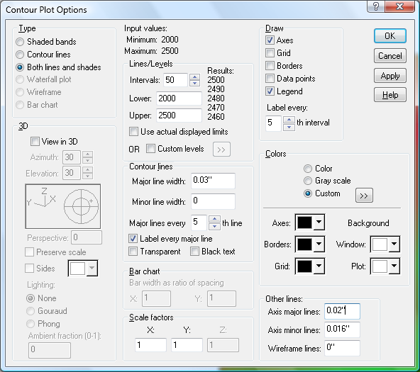
"Borders" and "Draw points" have been turned on to illustrate the bigger problem with both of these "average" reports: The average (or $MEAN) is simply an average of all values with no consideration given to the spacing between points. Just guessing, but that's probably not what you want since every point has an equal weight in determining the "average" as every other point, regardless of the area affected. What you need is a rectangular grid with evenly-spaced points in the X and Y directions. Select Options>Generate Mesh to produce a grid with evenly-spaced points:

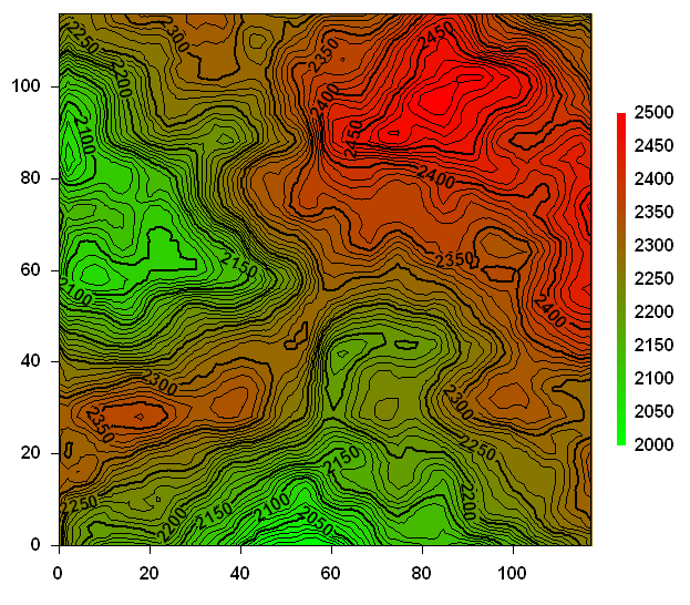
There's no magic involved in setting the number of intervals; any value that produces new points at a higher frequency than your original data will give a more realistic answer than your original plot. The "Bivariate" interpolation scheme generally results in a smoother surface than "Planar", but unless you have a good insight into your data there is usually no justification for using anything more complex than "Planar". The resulting plot, with the options shown above:

The $MEAN value shown here (which will now match the status bar value unless/until you zoom) is a much better guess at an "average" Z.
For your second question: "... or to integrate an area to directly compute the total lumen energy applied there?": Sure. Use Generate>Find Volume Under Surface to... well... find the volume under the surface. This is numerically equivalent to integrating the surface.

If you divide the volume given by that dialog (4272.45) by the total area (2500) you get an "average" Z value of 1.70898, slightly different than the $MEAN value of 1.733036. The difference is due to the $MEAN calculation giving equal weight to all data points, including those along the edges of the surface. Which value is more useful for your particular application? I have no idea :-). Different applications will have different answers.